RL - Introduction to Reinforcement Learning

RL, especially DRL (Deep Reinforcement Learning) has been an fervent research area during these years. One of the most famous RL work would be AlphaGo, who has beat Lee Sedol, one of the best players at Go, last year. And in this year (2017), AlphaGo won three games with Ke Jie, the world No.1 ranked player. Not only in Go, AI has defeated best human play in many games, which illustrates the powerful of the combination of Deep Learning and Reinfocement Learning. However, despite AI plays better games than human, AI takes more time, data and energy to train which cannot be said to be very intelligent. Still, there are numerous unexplored and unsolved problems in RL research, that's also why we want to learn RL.

This is the first note of David Silver's RL course.

About Reinforcement Learning
The Reinforcement Learning Problem
Inside An RL Agent
Problems within Reinforcement Learning

About Reinforcement Learning

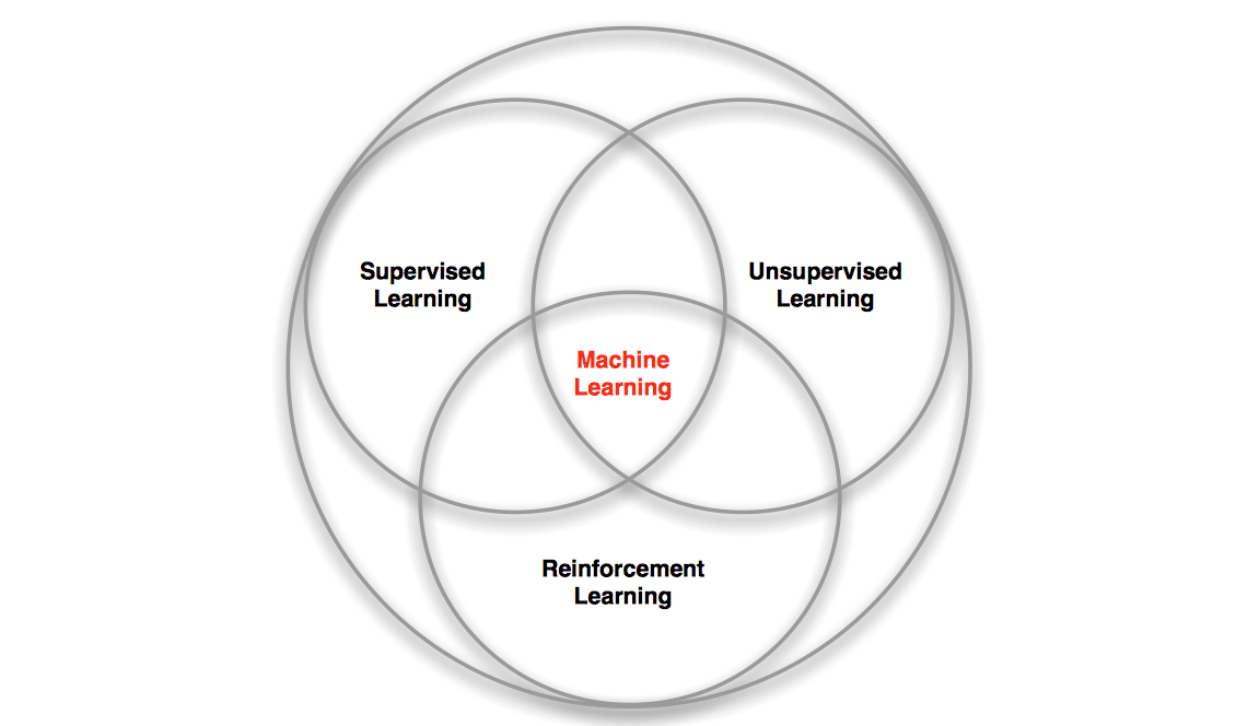
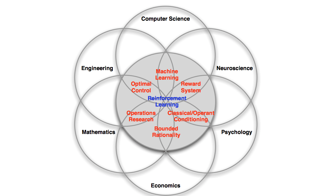
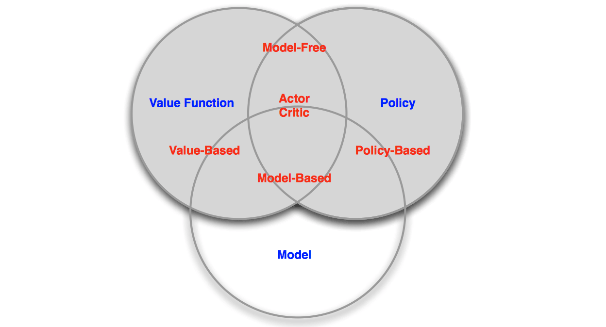
Reinforcement Learning is one of the three major branches of Machine Learning, and is also the intersect of many different disciplines, as the following two figure illustrated.

There are several reasons that makes reinforcement learning different from other machine learning paradigms:

There is no supervisor, only a reward signal
Feedback is delayed, not instantaneous
Time really matters (sequential, non i.i.d data)
Agent's actions affect the subsequent data it receives

There are some examples of Reinforcement Learning:

Fly stunt manoeuvres in a helicopter
Defeat the world champion at Backgammon
Manage an investment portfolio
Control a power station
Make a humanoid robot walk
Play many diﬀerent Atari games better than humans

The Reinforcement Learning Problem

Rewards

We say RL do not have a supervisor, just a reward signal. Then what is reward ?

A reward $R_t$ is a scalar feedback signal
Indicates how well agent is doing at step $t$
The agent's job is to maximise cumulative reward

Reinforcement Learning is based on the reward hypothesis, which is

Definition of reward hypothesis

All goals can be described by the maximisation of expected cumulative reward.

There are some examples of rewards :

Fly stunt manoeuvres in a helicopter
- +ve reward for following desired trajectory
- −ve reward for crashing
Defeat the world champion at Backgammon
- +/−ve reward for winning/losing a game
Manage an investment portfolio
- +ve reward for each $ in bank
Control a power station
- +ve reward for producing power
- −ve reward for exceeding safety thresholds
Make a humanoid robot walk
- +ve reward for forward motion
- −ve reward for falling over
Play many diﬀerent Atari games better than humans
- +/−ve reward for increasing/decreasing score

Sequential Decision Making

So, according to the reward hypothesis, our goal is to select actions to maximise total future reward. Actions may have long term consequences as well as reward may be delayed. It may be better to sacrifice immediate reward to gain more long-term reward. For instance, a ﬁnancial investment may take months to mature and a helicopter might prevent a crash in several hours.

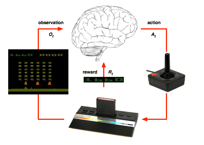
Agent and Environment

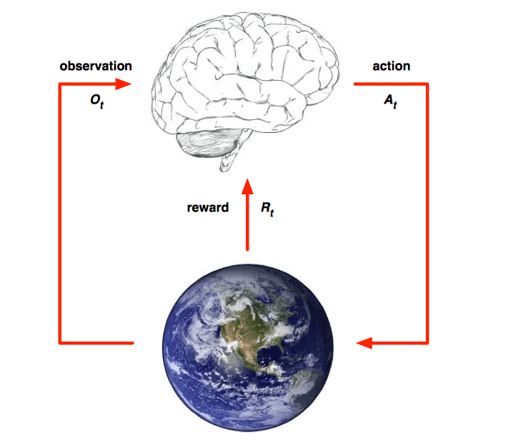
Agents and envrionments are big concepts in RL. They have following relationships:

At each step $t$ the agent:
- Excutes action $A_t$
- Receives observation $O_t$
- Receives scalar reward $R_t$
The environment:
- Receives action $A_t$
- Emits observation $O_{t+1}$
- Emits scalar reward $R_{t+1}$
$t$ increments at env. step

State

History and State

The history is the sequence of observations, actions, rewards: \[ H_t = O_1, R_1, A_1, ..., A_{t-1}, O_t, R_t \] which means all observable variables up to time $t$, i.e. the sensorimotor stream of a robot or embodied agent.

What happens next depends on the history:

The agent selects actions
The environments select observations/rewards

State is the information used to determine what happens next. Formally, state is a function of the history: \[ S_t = f(H_t) \] Environment State

The environment state $S^e_t$ is the environment's private representation, i.e. whatever data the environment uses to pick the next observation /reward. The environment state is not usually visible to the agent. Even if $S^e_t$ is visible, it may contain irrelevant information.

Agent State

The agent state $S^a_t$ is the agent's internal representation, i.e. whatever information the agent uses to pick the next action. It is the information used by reinforcement learning algotithms. It can be any function of history: \[ S^a_t=f(H_t) \] Information State

An information state (a.k.a. Markov state) contains all useful information from the history.

Definition

A state $S_t$ is Markov if and only if \[ P[S_{t+1}|S_t]=P[S_{t+1}|S_1,...,S_t] \]

The above formular means:

"The future is independent of the past given the present" \[ H_{1:t}\rightarrow S_t\rightarrow H_{t+1:\infty} \]
Once the state is known, the history may be thrown away.
The state is a sufficient statistic of the future
The environment state $S^e_t$ is Markov
The history $H_t$ is Markov

Rat Example

Here is an example to explain what is state, imagine you are a rat and your master would decide whether to excuted you or give you a pice of cheese. The master makes decisions according to a sequence of signals, the first two sequence and the result are shown in the figure below:

The question is, what would you get if the sequence is like below:

Well, the answer you may give is decided by what is your agent state：

If agent state = last 3 items in sequence, then the answer would be being excuted.
If agent state = counters for lights, bells and levers, then the answer would be given a piece of cheese.
What if agent state = complete sequence?

Fully Observable Environments

Full observability: agent directly observes environment state: \[ O_t = S^a_t=S^e_t \]

Agent state = environment state = information state
Formally, this is a Markov decision process (MDP)

Partially Observable Environments

Partial observability: agent indirectly observes environment:

A robot with camera vision isn't told its absolute location
A trading agent only observes current prices
A poker playing agent only observes public cards

With partial observability, agent state ≠ environment state, formally this is a partially observable Markov decision process (POMDP).

In this situation, agent must construct its own state representation $S^a_t$, e.g.

Complete history: $S^a_t = H_t$
Beliefs of environment state: $S_t^a = (P[S^e_t=s^1], …, P[S^e_t=s^n])$
Recurrent neural network: $S^a_t=\sigma(S^a_{t-1}W_s+O_tW_o)$

Inside An RL Agent

There are three major components of an RL agent, actually, an agent may include one or more of these:

Policy: agent's behaviour function
Value function：how good is each state and/or action
Model：agent's representation of the environment

Policy

A Policy is the agent's behaviour, it is a map from state to action, e.g.

Deterministic policy：$a = \pi(s)$
Stochastic policy: $\pi(a|s)=P[A_t=a|S_t=s]$

Value Function

Value function is a prediction of future reward, it is used to evaluate the goodness/badness of states. And therefore to select between actions: \[ v_\pi(s)=E_\pi[R_{t+1}+\gamma R_{t+2}+\gamma^2R_{t+3}+...|S_t=s] \] Model

A model predicts what the environment will do next, denoted by $P$ which predicts the next state and by $R$ predicts the next (immediate) reward: \[ P^a_{ss'}=P[S_{t+1}=s'|S_t=s,A_t=a] \]

\[ R^a_s=E[R_{t+1}|S_t=s, A_t=a] \]

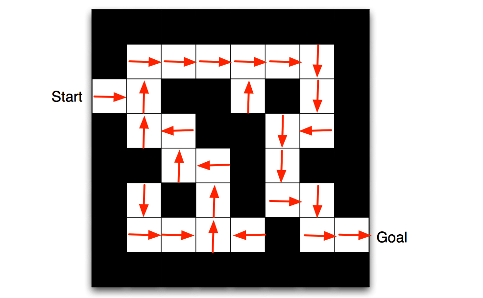
Maze Example

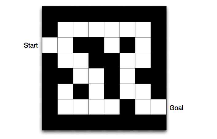
Let an RL agent to solve the maze, the parameters are:

Rewards: -1 per time-step
Actions: N, E, S, W
States: Agent's location

Then the policy map would be (arrows represent policy $\pi(s)$ for each state $s$):

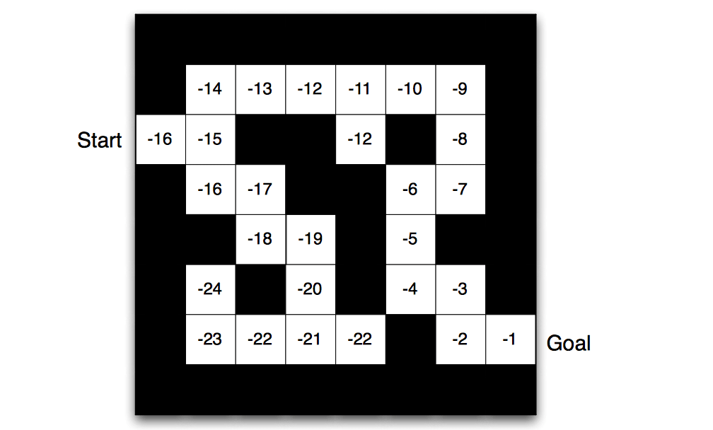
And the value function at each state would be (numbers represent value $v_\pi(s)$ of each state $s$):

Model could be visualize as following:

Grid layout represents transition model $P^a_{ss'}$
Numbers represent immediate reward $R^a_s$ from each state $s$ (same for all $a$)

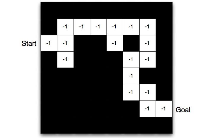
Agent may have an internal model of the environment
Dynamics: how actions change the state
Rewards: how much reward from each state
The model may be imperfect

Categorizing RL agents

RL agents could be categorized into several categories:

Value Based
- No Policy (Implicit)
- Value Function
Policy Based
- Policy
- No Value Function
Actor Critic
- Policy
- Value Function
Model Free
- Policy and/or Value Function
- No Model
Model Based
- Policy and/or Value Function
- Model

Problems within Reinforcement Learning

This section only proposes questions without providing the solutions.

Learning and Planning

Two fundamental problems in sequential decision making:

Reinforcement Learning
- The environment is initially unknown
- The agent interacts with the environment
- The agent improves its policy
Planning:
- A model of the environment is known
- The agent performs computations with its model (without any external interaction)
- The agent improves its policy a.k.a. deliberation, reasoning, introspection, pondering, thought, search

Atari Example: Reinforcement Learning

In atari games, rules of the game are unknown, the agent learns directly from interactive game-play by picking actions on joystick and seeing pixels and scores.

Atari Example: Planning

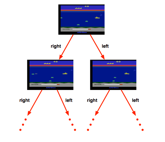
In such case, rules of the game are known, which means the agent could query the emulator as known as a perfect model inside agent's brain. Agents need plan ahead to ﬁnd optimal policy, e.g. tree search.

Exploration and Exploitation

Reinforcement learning is like trial-and-error learning
The agent should discover a good policy
From its experiences of the environment
Without losing too much reward along the way
Exploration ﬁnds more information about the environment
Exploitation exploits known information to maximise reward
It is usually important to explore as well as exploit

Examples

Restaurant Selection
- Exploitation Go to your favourite restaurant
- Exploration Try a new restaurant
Online Banner Advertisements
- Exploitation Show the most successful advert
- Exploration Show a diﬀerent advert
Game Playing
- Exploitation Play the move you believe is best
- Exploration Play an experimental move

Prediction and Control

Prediction: evaluate the future

Given a policy

Control: optimise the future

Find the best policy

End. Next note will introduce the Markov Decision Processes.